![]()

CORONAVIRUSES AND COVID-19
APPENDIX A
Pandemics
Dr Richard Hunt
Professor
Department of Pathology, Microbiology and Immunology
University of South Carolina School of Medicine
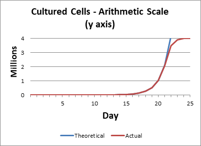 Figure 1A
 Cells in a tissue culture flask approximately double each day (blue line). However, they will run out of space and nutrients as they cover the plate and the division rate will tail off giving us a sigmoid growth curve (red line).
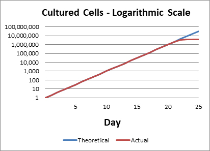 Figure 1B
When we plot of the cell number on a logarithmic axis, we can see that until
cell proliferation tails off, the cell number is increasing logarithmically.
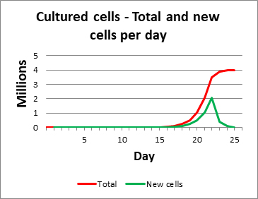 Figure 1c
The slope of our sigmoid curve represents the number of new cells each
day which falls as the proliferation tails off.
Epidemic
A widespread occurrence of an infectious disease in a community at a particular time.Pandemic
A type of epidemic but one with greater range and coverage or an outbreak of a disease that occurs over a wide geographic area and affects an exceptionally high proportion of the population. While a pandemic may be characterized as a type of epidemic, you would not say that an epidemic is a type of pandemic.
Source: Merriam-Webster Dictionary
An exponential increase in numbers
Why does the number of cases rise rapidly in an epidemic or pandemic?
At a beginning of an epidemic, we first see a few isolated cases in the population and most people are, of course, uninfected. Clusters of infected patients develop, each seeded by a single infected person (patient zero); but after a period of time that depends on the contagiousness of the virus, many people become infected with ever-increasing numbers of new cases each day. This often seems to happen almost overnight. And then things usually level off and the number of new cases starts to decline. Why does this happen?
The sudden increase in the number of infected people
results from the fact that infections increase exponentially
(logarithmically) rather than linearly.
Exponential (logarithmic) growth
Consider a single cell in a plastic tissue culture dish. In our example, the cells divide, on average, every day. After one day, there will be two cells; after two days four; after three days eight etc. Even by day 7, there are only 128 cells. The increase in the number of cells is shown in figure 1a (blue line). When we plot the number of cells with a logarithmic scale on the ordinate (y) axis, we can see that the cells are proliferating logarithmically or exponentially (figure 1b - blue line).
However, division cannot go on forever and the cells will stop dividing when they cover the plate (i.e. they become confluent), on day 22 in our example. Note that, during our 22 day division process, the cells cover just 0.025% of the plate at day 10, and 1% of the plate between days 15 and 16. They still cover under 5% of the plate around day 17, just 50% on day 21 and all of the plate (i.e. they are fully confluent) only on day 22. At this point they must stop growing as there is no plate left to cover.
The cells do not stop dividing abruptly, however, as factors such as the depletion of the medium will cause the growth rate to slow. Thus, the initially logarithmic proliferation of the cells tails off and our curve becomes sigmoid, as shown in figure 1a (red line). However, during the initial rise of the cell number in our sigmoid curve, proliferation is still logarithmic (figure 1b (red line)).
In figure 1a, the slope of the red line indicates the number of new cells per day. This is shown in figure 1c (green line).
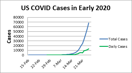 Figure 2a
The number of COVID-10 cases in the United States in early 2020. The total
number of cases (blue line) and the number of new cases each day (green
line) are shown.
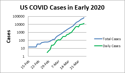 Figure 2b
On a logarithmic scale, initially the total and new cases rose
exponentially.
The situation in an infectious disease
So now let’s turn to the case of a disease epidemic. In a naïve population in which no one is vaccinated or has any pre-existing immunity, infectious diseases spread logarithmically (exponentially). In a pandemic, we first see clusters of cases, each seeded by a single person (a patient zero). Thus, when COVID-19 broke out in China, the virus presumably skipped to one person from pangolins, bats or some other yet to be identified host. At first, the disease went unnoticed because very few people showed up at clinics but then more and more people exhibited similar symptoms and an exponential increase was on the way. The same thing happened in western countries: First, there were just a few COVID-19 patients and then there were many and the numbers were doubling every few days.
Thus, infectious diseases progress in the same way as our cultured cells: logarithmically. In the beginning, only a few people appear to be infected and then suddenly the numbers rise precipitously. Figure 2a shows the total number of cases of COVID-19 in the United States in the first part of 2020 and the number of new cases each day. Again, the total number of cases rise logarithmically (figure 2b). We do not know exactly when the disease entered the US population but it was probably seeded by a number of travelers from outside, probably from China and Europe and so localized hot spots appeared. Thus, there was no one US Patient Zero.
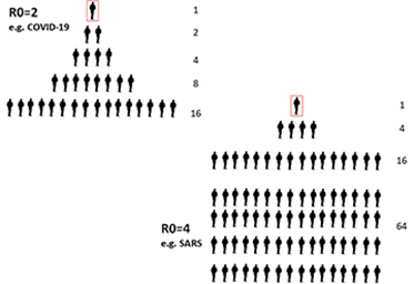 Figure 3
R0 (reproduction number) is the average number of uninfected people infected by one infected person; for example, SARS-CoV-2 (the virus that causes COVID-19) has an R0 of around two and so, on average, a person who has COVID-19 will pass the virus on to two other people (left). SARS-CoV, the virus that caused the original SARS epidemic, is more contagious with an R0 of about four and so an infected person will pass, on average, the virus to four other people.
Basic Reproduction Factor (R0)
If the disease is contagious, each infected person may infect more than one person and this is shown in figure 3. In the case of COVID-19, it was estimated that each infected person, on average, is likely to pass the virus to two people during the period that the original person is infectious. This means that SARS Co-2, the virus that causes COVID-19, is not as infectious as many other viruses. In contrast, the virus that caused the original SARS outbreak in China was more infectious and it is estimated that each infected person could pass the virus to, on average, four people.
This leads us to the idea that each virus has a reproduction number (or reproduction factor) that represents the degree of infectivity of that particular virus. This is a very approximate measure since the degree of contagion will differ with the circumstances of the disease outbreak but it does also reflect the properties of the virus itself.
Epidemiologists often refer to the infectivity or reproduction number of a virus as its R0 (R naught). R0 is a mathematical term that indicates how contagious an infectious disease is. In epidemiology, the reproduction number of an infection is the expected number of cases directly generated by one case in a population where all individuals are susceptible to infection; that is when no one is immune to the disease by prior exposure or vaccination.
Figures 4a and b show the kinetics of infection at the early stages of an epidemic when an infected person infects 1, 1.05, 2 and 4 other people. The original person then either recovers from the infection (and therefore is not an active case) or dies.
In figure 4a, we can see just how much more infectious a virus with an R0 of 4 is than one with an R0 of 2. In the case of the R0 of 2, the number of cases merges into the X-axis. These data are shown more informatively on a logarithmic scale in figure 4b. We can see that in all cases of an R0 of more than 1, the number of cases rises logarithmically but at different rates.
What we need to know for a given disease is how contagious the disease is. That is, on average how many people an infected person will infect before the original infected person stops being infectious. Clearly, some viral diseases are more contagious than others and this mostly depends on how they are transmitted. For example, influenza can be transmitted on water droplets when someone coughs or sneezes. It can also be spread indirectly by contact with surfaces onto which someone has sneezed (these are called fomites and could be clothes, cups, the surfaces of benches, taps etc.). The length of time that a virus can remain infectious depends on many factors including the properties of the virus (whether enveloped or non-enveloped, for example) and the nature of the surface. Influenza virus can survive on some surfaces for up to 2 days.
This means that it is quite hard to avoid influenza viruses as we see every winter. In contrast, HIV and Ebola are spread in a different way. HIV is mainly spread by sexual contact, contaminated needles etc. while Ebola is spread by contact with blood, urine etc. from an infected patients. Thus, by simple precautions, we can avoid the spread of HIV or Ebolavirus but it is much more difficult to avoid the flu, especially in crowded environments.
One of the more contagious viruses is measles which is spread by water droplets in the air after a cough or sneeze by an infected person. In fact, it is likely that every non-vaccinated person in a room will contract the disease from one infected person. Moreover, the air-borne virus may remain viable for some time. Measles replicates initially in the upper/lower respiratory tract, followed by replication in lymphoid tissues leading to viremia and growth in a variety of epithelial sites. The disease develops 1 - 2 weeks after infection but an infected person can be contagious four or more days before the rash symptoms appear. Thus, an infected person may not know that they are infected although eventually almost every infected person does show symptoms which make eradication much easier. Some virus shedding also continues to occur during the overt disease phase and may continue for four or more days after the rash goes away.
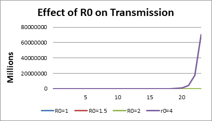 Figure 4a
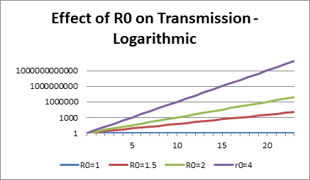 Figure 4b
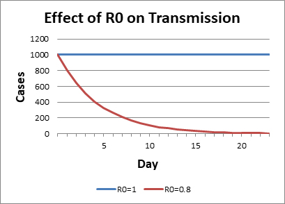 Figure 5a
When R0 is less than 1, that is when one person transmits the infection to
less than one person when the former is infected, the infection tails out
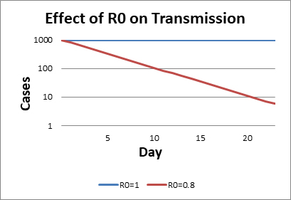 Figure 5b
The infection tails out logarithmically
Here are some R0 values for viruses that are spread by airborne droplets:
Measles ~12
Mumps ~5
Smallpox ~5
SARS 2-5
COVID-19 1.5-4
Seasonal flu 1-2
1918 pandemic flu (Spanish flu) 1.4-2.8
MERS 0.3-0.8
The difference in R0 or infectivity of the various airborne viruses depends on a number of factors:
The length of time the infected patient is infectious
The number of infectious viruses that the patient produces and the level of viremia that the patient experiences
Whether there is a prodromal period in which there are no symptoms and therefore the patient does not know if they are infected
Whether, as in measles, the patient sheds infectious virus after the resolution of overt symptoms
The stability of the virus
So, as seen in figure 4, if the R0 for the virus is more than 1, each infected person will infect more than one uninfected person and the number of infected people will expand, i.e. an epidemic will ensue. The higher the R0, the more rapidly the epidemic will progress; that explains why measles spreads so rapidly.
If the R0 of the virus is around 1, each infected person will each infect one other person. Since, in the case of most viral infections, the infected person gets immunity and the virus goes away, the disease will remain in the population but there will be no epidemic and no rapidly rising number of cases.
If the R0 is less than one, the virus is not very infectious. Thus, if a thousand people (for example) only infect perhaps eight hundred other people before the disease is cured in the original thousand and so on, the disease will peter out (figure 5a and b). Note, for example, that MERS-CoV has a low R0 (less than 1) and this is exactly what seems to have happened with the MERS outbreak in Saudi Arabia that started in 2012. The virus is still around but no epidemic has ensued even though there is no vaccine for MERS.
Case Fatality Rate
Note that the R0 (infectivity) of a virus is not the same as the case fatality (mortality) rate (ratio), often referred to as the CFR. The case fatality rate for a disease is the number of fatalities divided by the number of confirmed infections. Although the R0 of MERS is low, many people infected with MERS-CoV developed severe respiratory illness similar to COVID-19, including a dry cough, shortness of breath and a fever. Many of these MERS patients have died with an apparent case-fatality rate of around 34%. Whether the fatality rate is this high, however, is uncertain as many milder cases may go undetected.
Here are the case mortality rates for the above air-borne viruses in the absence of vaccination. These rates are approximate as the fatality rate in the case of measles is very dependent on such factors as nutritional status and therefore mortality is much higher in malnourished children and where health care is poor:
Measles 1-3%
Mumps 1%
Smallpox (Variola major) 30% Variola minor 1%
SARS >11%
MERS 34%
COVID-19 ~1.4%* (Data for China: Lancet April 2020)
Seasonal flu 0.1%
1918 pandemic flu (Spanish flu) >2.5%
* This crude CFR may be artificially high whereas that for seasonal flu is much more accurate as it has been around for a very long time and testing has been much more intensive in many countries.
Although the mortality rate of measles is low, it is so contagious that before the introduction of measles vaccine in 1963, major epidemics occurred approximately every 2 to 3 years resulting in an estimated 2.6 million deaths each year. Even with the current excellent vaccine, in 2018 there were more than 140,000 measles deaths around the world, mainly in children under five years of age.
Here are the CFRs for SARS, COVID-19 and seasonal flu.
|
Case fatality rate for SARS, COVID-19 and seasonal influenza |
|||
|
|
SARS |
COVID-19 |
Influenza |
|
Overall |
14-15% |
1.38% |
0.096% |
|
0-4 years |
0 |
0.0026 |
0.0073 |
|
18-19 |
|
|
0.02 |
|
20-24 |
|
0.06 |
|
|
25-29 |
1.6 |
|
|
|
30-34 |
|
0.15 |
|
|
40-44 |
|
0.3 |
|
|
45-49 |
13 |
|
|
|
50-54 |
|
1.25 |
0.06 |
|
55-59 |
25 |
|
|
|
60-64 |
|
4.0 |
|
|
65-69 |
53 |
|
0.8 |
|
70-74 |
|
8.6 |
|
|
75-79 |
70 |
|
|
|
>80 |
|
13 |
|
|
Data from: Shigui Ruan Likelihood of survival of coronavirus disease 2019. Lancet March 30, 2020 DOI:https://doi.org/10.1016/S1473-3099(20)30257-7 |
|||
CFRs can be highly variable from country to country and within a country; for example, when COVID-19 broke out in Wuhan, China, the CFR was high The overall CFR varies by location and intensity of transmission (i.e. 5.8% in Wuhan vs. 0.7% in other areas in China). Initially (early January, 2020), the CFR in China was 17.3% but this was reduced to 0.7% by early February as the standard of care evolved over the course of the outbreak (Report of the WHO-China Joint Mission via worldometers.info).
Effective Reproduction Factor (Rt) and Herd Immunity
R0 numbers only apply when the population is naïve; that is when there has been no vaccination and no immunity in the population resulting from prior exposure. When there is no way to control the spread of the disease using chemotherapy or vaccination, the best way to reduce the severity of the epidemic is to reduce the R0 by non-pharmaceutical interventions such as quarantine, “social distancing” and other methods of interfering with spread such as hand washing, disinfectants and masks. The R0 can vary from one location to another because of the population’s age structure and the frequency with which people come into close contact with one another. For example, people are in much closer together in large cities compared to rural locations.
So far, we have seen that a disease can spread exponentially in a naïve population. But it cannot spread forever as it will run out of people to infect just as our tissue culture cell ran out of nutrients and space. As we saw, exponential culture cell proliferation does not end abruptly for a number of reasons but it tails off after the logarithmic phase so that the number of cells reaches a plateau and the proliferation curve is sigmoid. The same happens in the spread of an epidemic. Eventually, the spread of the disease tails off and it does not do so when 100% of the susceptible population is infected. Sooner or later, the R0 will go down since, as the number of infected people in the population rises, the virus will find it harder and harder to find someone to infect. In addition, in the real disease situation, people do not remain infected forever as they develop immunity or, in some cases, die. Thus, we see a sigmoid progression of the disease numbers. The fact that not all the people in the community get the infection is because of what is known as herd immunity. As more and more people become immune to the disease as a result of their immune response, the infected people fail to meet uninfected people while the former are infectious. This is why we need only to vaccinate 60-70% of the population to stop a disease from progressing.
So here is what we get with a disease that is caused by a virus with an R0 of 2 (figure 6)
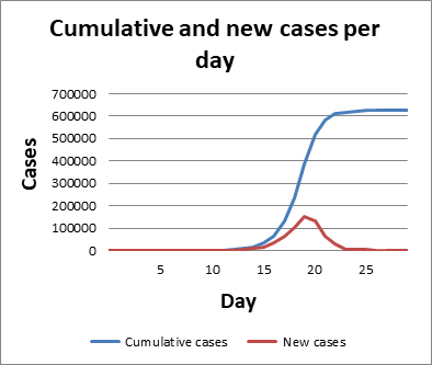 Figure 6
The time course of an infectious disease with a doubling of infection every day
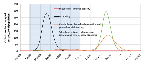 Figure 7
Imperial College London: Impact of Public Health Measures on the COVID-19
Pandemic predictions and scenarios for the UK showing intensive care unit
(ICU) requirements.
Black: Unmitigated epidemic.
Green: Suppression strategy incorporating closure of schools and
universities, case isolation and population-wide social distancing beginning
in late March 2020.
Orange: Containment strategy incorporating case isolation, household
quarantine and population-wide social distancing.
Blue shading: 5-month period in which these interventions are assumed to
remain in place
(Source: WHO collaborating Centre / MRC GIDA / J-IDEA
Note that here, the rate of the increase in infected people (that is the slope of the sigmoid curve) gives us the number of new cases each day and we get a bell-shaped curve.
Thus, R, the reproduction number, can vary during an epidemic, first because of population dynamics, for example the proportion of the population who are infected and also by interventions such as social distancing. Thus, the effective reproduction number can be referred to as Rt, the reproduction number or transmission rate at a given time. This is a much more useful number as it changes as controls are brought in to counteract an epidemic. Such controls could be testing and quarantine, restrictions on movement (“shelter in place”), the closing of schools, restaurants, bars and non-essential shops, the wearing of face masks, hand washing, decontamination of surfaces etc.
Figure 7 is our most important curve as it relates directly to the elimination of the disease from the population. Clearly, it is important in any disease outbreak to slow the number of new cases so that they do not overwhelm the medical resources available. Indeed, what spurred several countries to act in a more decisive manner was the prediction of what would happen when if COVID-19 went unchecked. As can be seen in this graph, left unchecked, medical facilities would be totally overwhelmed, as indeed they have been in Italy. The curve is flattened, i.e. the Rt is lowered by testing for and quarantining infected people, closing schools, universities and other places where people congregate, social distancing etc. This is exactly what China did to an extreme degree when the rise of COVID-19 became apparent. Early models of the disease’s spread, which did allow for containment efforts, suggested that SARS-CoV-2, would infect about 500 million people (40% of the Chinese population). Note that with extensive containment including testing, isolation, quarantine and social distancing as well as school and university closings, the number of cases remains below the capacity of the health system (critical care beds). However, once the restrictions are lifted the pandemic resumes once again. Indeed, the second wave is worse that if nothing had been done at all because many fewer people had contracted the disease in the first wave and so there are many more people in the population that have no immunity. This is why herd immunity was considered (but rejected) by most countries. So why bother to initiate the restrictions in the first place if they only delay the pandemic? Certainly, the restrictions cannot remain in force indefinitely. The answer is that the restrictions allow us to buy time to search for drug treatments and vaccines and to educate the public about social distancing and the use of masks. Most importantly, they allow a test, track and quarantine system to be set up. With a successful system, it is hoped that the second wave may be reduced to manageable levels.
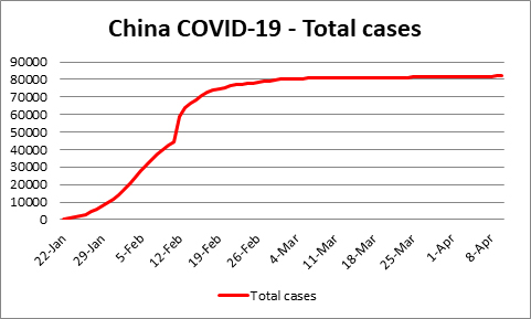 Figure 8a.
Cases of COVID-19 recorded in China, Spring 2020
China
In mid-January, Chinese authorities took extreme measures to contain the SARS-CoV-2 infections. They stopped all movement in and out of Wuhan, the capital of Hubei province and the epicenter of the epidemic, and fifteen other cities in Hubei province which is home to more than 60 million people (January 16). A little later, the inhabitants of many Chinese cities were instructed to remain in their homes and only venture out for food or medical help. As a result about 760 million people, roughly half the country’s population, were confined to their homes, according to The New York Times. And, indeed it worked. It appears that the Rt had been reduced to 1.05 and new and active cases leveled off in late February and then fell rapidly (Figure 8a and b). The number of new cases in China reached a peak around February 2. By mid to late March, China was reporting no new domestic cases each day, the few new cases being imported as Chinese residents returned home.
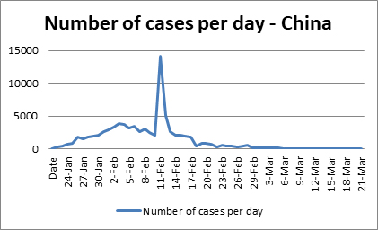 Figure 8b.
The number of new cases of COVID-19 each day recorded in China, Spring 2020
Note there is a spike on February 11/12. This was not a sudden rise in new cases but a change in the way cases were recorded. The sharp rise in cases was due to a new case definition that included both laboratory-confirmed cases and clinically diagnosed cases. Previously, only laboratory-confirmed courses had been recorded.
What happens when restrictions are lifted?
Thus, lowering the curve can be achieved by rapid testing and quarantining and stopping social interactions that lead to the spreading of infection. The aim is to lower the peak of the curve and to spread out the cases of infection over a longer time so that medical facilities are not overwhelmed. Nevertheless, once non-pharmaceutical interventions are relaxed, the majority of the population will still be at risk of infection and the number of new cases will inevitably increase once again (figure 7). Because of the economic damage of strict “stay-at-home” policies, it is unlikely that by the time restrictions are lifted, better methods of treating the disease will have been discovered and progress towards a vaccine will have been made. Thus, it is imperative that non-pharmaceutical interventions are maintained. These include social distancing and barriers to infection such as the use of masks in public, especially crowded situations.
The effects of high mask usage are discussed in this section.
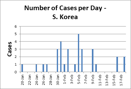 Figure 9a
Up to February 18, there were just 32 cases of COVID-19 in South Korea
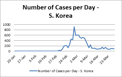 Figure 9b
However, the numbers rose precipitously as a result of the infection of a
church congregation by patient 31
South Korea
An interesting case of an outbreak where we do know the source occurred in South Korea. Early in the COVID-19 epidemic, South Korea tested tens of thousands of people per day in order to isolate any infections. As a result of these aggressive measures, the country was able to stabilize the epidemic with 30 infections up to Sunday February 16 (figure 9a). However, on Monday February 17, 2020, a new case (patient 31) in a 61 year old woman appeared in the city of Daegu, well away from Seoul, the previous center of infection. This woman may have become infected in Seoul which she occasionally visited. The public health authorities has a policy of tracing the contacts of as many infected people as possible and it turned out that this woman had a lot of contacts who were identified and tracked by interviews, phone and credit card records, GPS phone tracking and video surveillance. She belonged to an obscure, rather secretive church in which the congregants, more than 1000 at one time, sit very closely during services. Thus, there were at least one thousand people in her close contacts. Although the disease had initially appeared stabilized with only 30 cases, South Korea recorded twenty new cases within a day (Tuesday). By Wednesday, February 26, there were over 1000 cases and the number was rising exponentially (figure 9b). At least half of the cases were linked directly to the patient’s church.
Patient 31 had complained of headaches as a result of a car accident and had gone to a hospital ten days before she was diagnosed with COVID-19. She had no indications that she might be infected with SARS-CoV-2 as she had none of the common symptoms but patients are often infectious before they exhibit any of the characteristic symptoms of the disease. While in hospital, she developed a fever and flu was suspected but the test turned out to be negative. Unfortunately, she then left the hospital to go to a church service on February 16. On February 17, she developed pneumonia and was confirmed to have a SARS-CoV-2 infection. Thus, she had been in hospital, on and off, for ten days before she developed the characteristic symptoms of the disease.
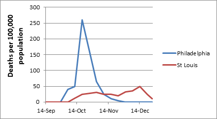 Figure 10. Comparison of the number of cases in St Louis, Missouri and
Philadelphia, Pennsylvania, Fall 2018.
Figure 10. Comparison of the number of cases in St Louis, Missouri and
Philadelphia, Pennsylvania, Fall 2018.A tale of two cities
Taking measures to lower the rate of person to person transmission of the virus has worked with Covid-19 in China. We also have an example of the success of lowering the curve from the 1918 Spanish flu epidemic. Incidentally, the designation of the 1918 pandemic as “Spanish” flu is a misnomer, as no evidence suggests the pandemic originated in that country or was more severe there than elsewhere. The first cases were detected in Europe and the US where the virus probably arose in Kansas and was spread to Europe by American soldiers. As Spain was neutral during the First World War, its media covered the epidemic there without restraint. The popular association of the 1918 pandemic with Spain (in name only) is thought to have arisen from that high-profile news coverage.
In 1918, returning soldiers and sailors brought the 1918 flu back to the United States. In Philadelphia, a hot spot of flu was the navy yard where about 600 sailors became sick. Soon after, there was to be a Liberty Bond parade in the city. This was not cancelled as the flu spread and about 200,000 people came together for the parade. The infection grew exponentially and 12,000 people died in the next six weeks. In the end, there were more than 500,000 cases in the city with 16,000 dead. In contrast, St Louis cancelled its parade and only 700 people in the city died.
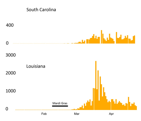 Figure 11.
Daily cases of COVID-19 in Louisiana and South Carolina, Spring 2020
New Orleans and Mardi Gras
Before the many of the United States enacted “stay at home” restrictions, the annual Mardi Gras celebrations took place in New Orleans, Louisiana in the last two weeks of February, Mardi Gras itself being on February 25. The close proximity of Mardi Gras celebrants probably led to a major increase in COVID-19 cases in that area. Cases rose at the beginning of March and peaked on April 2 (figure 11). Louisiana (4.6 million) has a similar population to South Carolina (5.1 million) but the latter did not see the major spike in cases in April (figure 11).
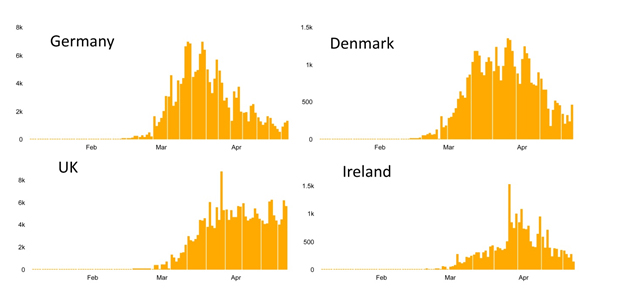 Figure 12. Comparison of the Covid-19 outbreaks in Germany, Denmark, the
United Kingdom and Ireland up to the beginning of May 2020.
Figure 12. Comparison of the Covid-19 outbreaks in Germany, Denmark, the
United Kingdom and Ireland up to the beginning of May 2020.Comparisons of different countries
Different countries put sever restrictions on movement and issued “stay at home” edicts at different times. The stay at home dates were: Ireland 12th March, 2020; Denmark 11th March, UK, 23rd March. In the case of Germany, lockdown was started in Freiburg, Baden-Württemberg and Bavaria on 20 March 2020. Three days later, it was expanded to the whole of Germany. Germany instituted better test, track and quarantine regimen than most other countries.
![]() Return to the Coronavirus page
Return to the Coronavirus page
![]() Return to the Virology section of Microbiology and Immunology On-line
Return to the Virology section of Microbiology and Immunology On-line
This page last changed on
Saturday, May 30, 2020
Page maintained by
Richard Hunt